Case Study 3.1: Exam by itself

Problem

We wish to investigate the distribution of exam marks. In particular, we want to test the hypothesis that the underlying mean value of exam score is the ``historical average’’ of 55.

The variable of interest is:

• Exam: Exam mark out of 100.

Question of Interest

We were interested in building a model to describe exam marks. In particular, we want to test the hypothesis that the underlying mean value of exam score is the ``historical average’’ of 55.

Read in and Inspect Data

Stats20x.df = read.table("STATS20x.txt", header = TRUE)
hist(Stats20x.df$Exam, xlab = "Exam", main = "")
summaryStats(Stats20x.df$Exam)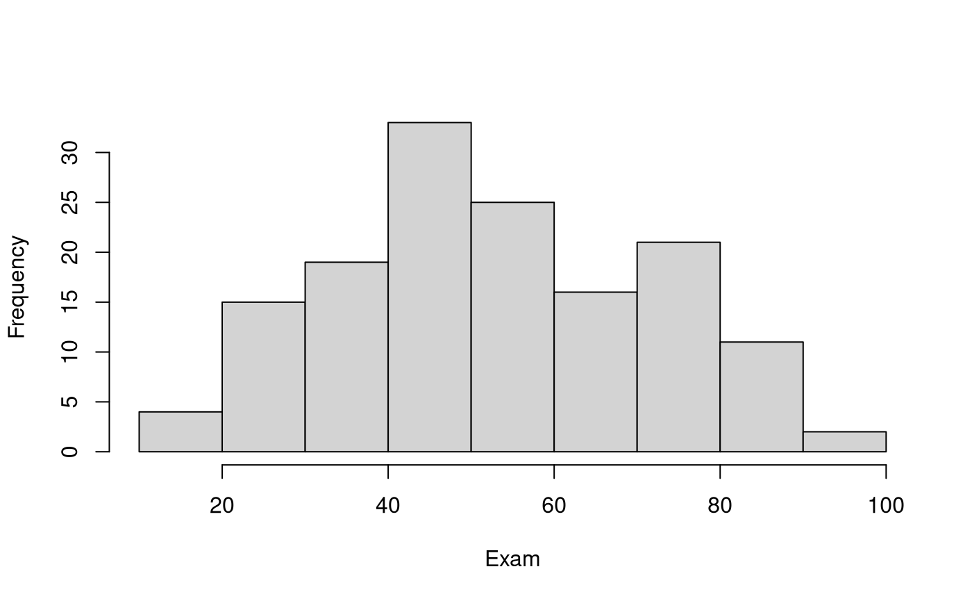

## Minimum value:           11 
## Maximum value:           93 
## Mean value:              52.88 
## Median:                  51.5 
## Upper quartile:          68.5 
## Lower quartile:          40 
## Variance:                348.87 
## Standard deviation:      18.68 
## Midspread (IQR):         28.5 
## Skewness:                0.16 
## Number of data values:   146

The exams marks are centred just above 50. The data look reasonably unimodal and symmetrical – roughly normal. Some slight right-skewness, but does not look like a problem.

Fitting the null model

By hand…

(mn_exam = mean(Stats20x.df$Exam)) # Sample mean

## [1] 52.87671

(sd_exam = sd(Stats20x.df$Exam)) # Sample standard deviation

## [1] 18.67799

(n_exam = length(Stats20x.df$Exam)) # Sample size

## [1] 146

(tmult_exam = qt(1 - 0.05 / 2, df = n_exam - 1)) # t-multiplier

## [1] 1.97646

(CI_exam = mn_exam + tmult_exam * c(-1, 1) * sd_exam / sqrt(n_exam)) # Confidence Interval

## [1] 49.82150 55.93193

(se_exam = sd_exam / sqrt(n_exam)) # Standard error

## [1] 1.545802

(t_stat_exam = (mn_exam - 55) / (se_exam)) # t-stat

## [1] -1.373583

(pval_exam = 2 * (1 - pt(abs(t_stat_exam), df = n_exam - 1))) # p-value

## [1] 0.171691

Using lm…

examNull.fit55 = lm(I(Exam - 55) ~ 1, data = Stats20x.df)
(pval_exam = coef(summary(examNull.fit55))[4])

## [1] 0.171691

55 + confint(examNull.fit55)

##               2.5 %   97.5 %
## (Intercept) 49.8215 55.93193

Finaly, with the t.test function

t.test(Stats20x.df$Exam, mu = 55)

## 
##  One Sample t-test
## 
## data:  Stats20x.df$Exam
## t = -1.3736, df = 145, p-value = 0.1717
## alternative hypothesis: true mean is not equal to 55
## 95 percent confidence interval:
##  49.82150 55.93193
## sample estimates:
## mean of x 
##  52.87671

Method and Assumption Checks

There are no explanatory variables, and so a null model was fitted.

From examining the histogram it appears that the data are roughly normally distributed, so model assumptions are satisfied.

Our final model is $$Exam_i=\beta_0 + \epsilon_i \text{ (or }Exam_i=\mu + \epsilon_i \text{)} ~,$$ where $\epsilon_i \sim iid ~ N(0,\sigma^2)$

Executive Summary

We were interested in building a model to describe exam marks.

We estimate the expected exam mark to be between 49.8 to 55.9 (out of 100).

We have no reason to believe that the expected exam mark differs from the historical average value of 55 (out of 100) (P-value = 0.17).