Case Study 8.1: Exam vs attendance and test mark • s20x

Problem

We’ve previously used test marks and attendance seperately in order to explain variability in exam marks. The objective here is to use them together.

Question of Interest

To quantify students’ exam marks relationship with attendance and test marks. Also, does any relationship between exam marks and test marks depend on whether students attended lectures.

Read in and Inspect the Data

Stats20x.df = read.table("STATS20x.txt", header = TRUE)
plot(Exam ~ Test,
  data = Stats20x.df, pch = substr(Attend, 1, 1), cex = 0.7,
  col = ifelse(Attend == "Yes", "blue", "red")
)

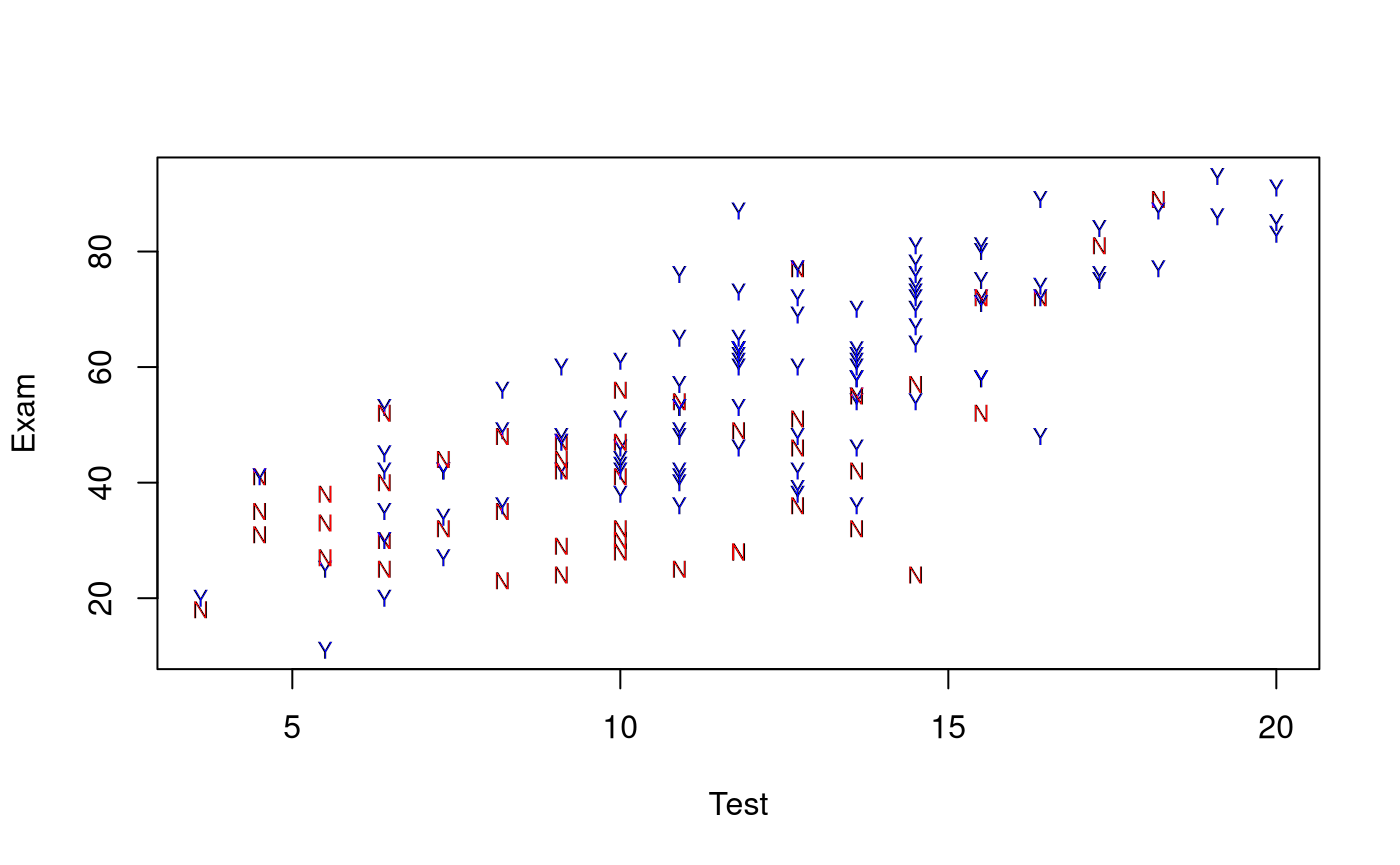
A scatter plot of test score versus exam suggested that the positive relationship between test and exam was reasonably linear within each attendance group (“Yes” or “No”), but that the slope could be different in the two groups.

Model Building and Check Assumptions

examTestAttend.fit = lm(Exam ~ Test * Attend, data = Stats20x.df)
plot(examTestAttend.fit, which = 1)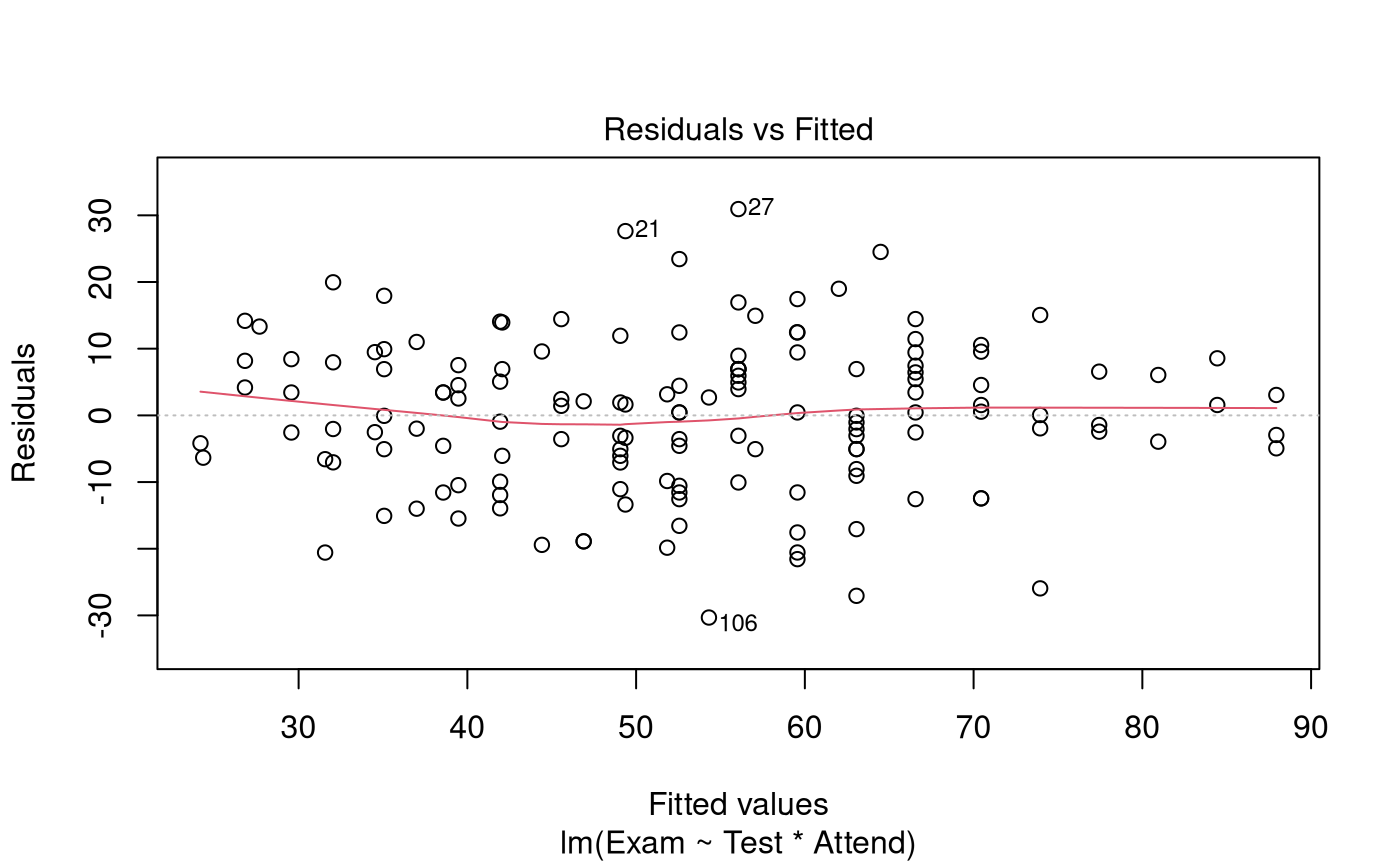

normcheck(examTestAttend.fit)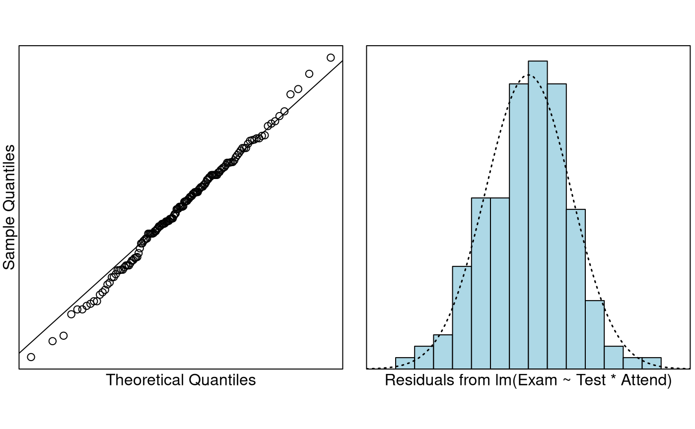

cooks20x(examTestAttend.fit)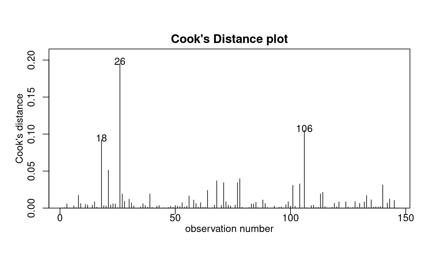

summary(examTestAttend.fit)

## 
## Call:
## lm(formula = Exam ~ Test * Attend, data = Stats20x.df)
## 
## Residuals:
##      Min       1Q   Median       3Q      Max 
## -30.3155  -6.5139   0.4383   7.3166  30.9383 
## 
## Coefficients:
##                Estimate Std. Error t value Pr(>|t|)    
## (Intercept)     14.4467     4.9443   2.922  0.00405 ** 
## Test             2.7496     0.4603   5.973 1.78e-08 ***
## AttendYes       -4.2582     6.3723  -0.668  0.50506    
## Test:AttendYes   1.1380     0.5577   2.040  0.04316 *  
## ---
## Signif. codes:  0 '***' 0.001 '**' 0.01 '*' 0.05 '.' 0.1 ' ' 1
## 
## Residual standard error: 11.41 on 142 degrees of freedom
## Multiple R-squared:  0.6347, Adjusted R-squared:  0.627 
## F-statistic: 82.25 on 3 and 142 DF,  p-value: < 2.2e-16

confint(examTestAttend.fit)

##                       2.5 %    97.5 %
## (Intercept)      4.67287511 24.220625
## Test             1.83956971  3.659567
## AttendYes      -16.85506294  8.338572
## Test:AttendYes   0.03547053  2.240510

Visualise the Final Model

predAttend.df = data.frame(Test = 1:21, Attend = "Yes")
predSlackers.df = data.frame(Test = 1:21, Attend = "No")
plot(Exam ~ Test,
  data = Stats20x.df, pch = substr(Attend, 1, 1), cex = 0.7,
  col = ifelse(Attend == "Yes", "blue", "red")
)
lines(1:21, predict(examTestAttend.fit, predAttend.df), col = "blue", lty = 2)
lines(1:21, predict(examTestAttend.fit, predSlackers.df), col = "red", lty = 2)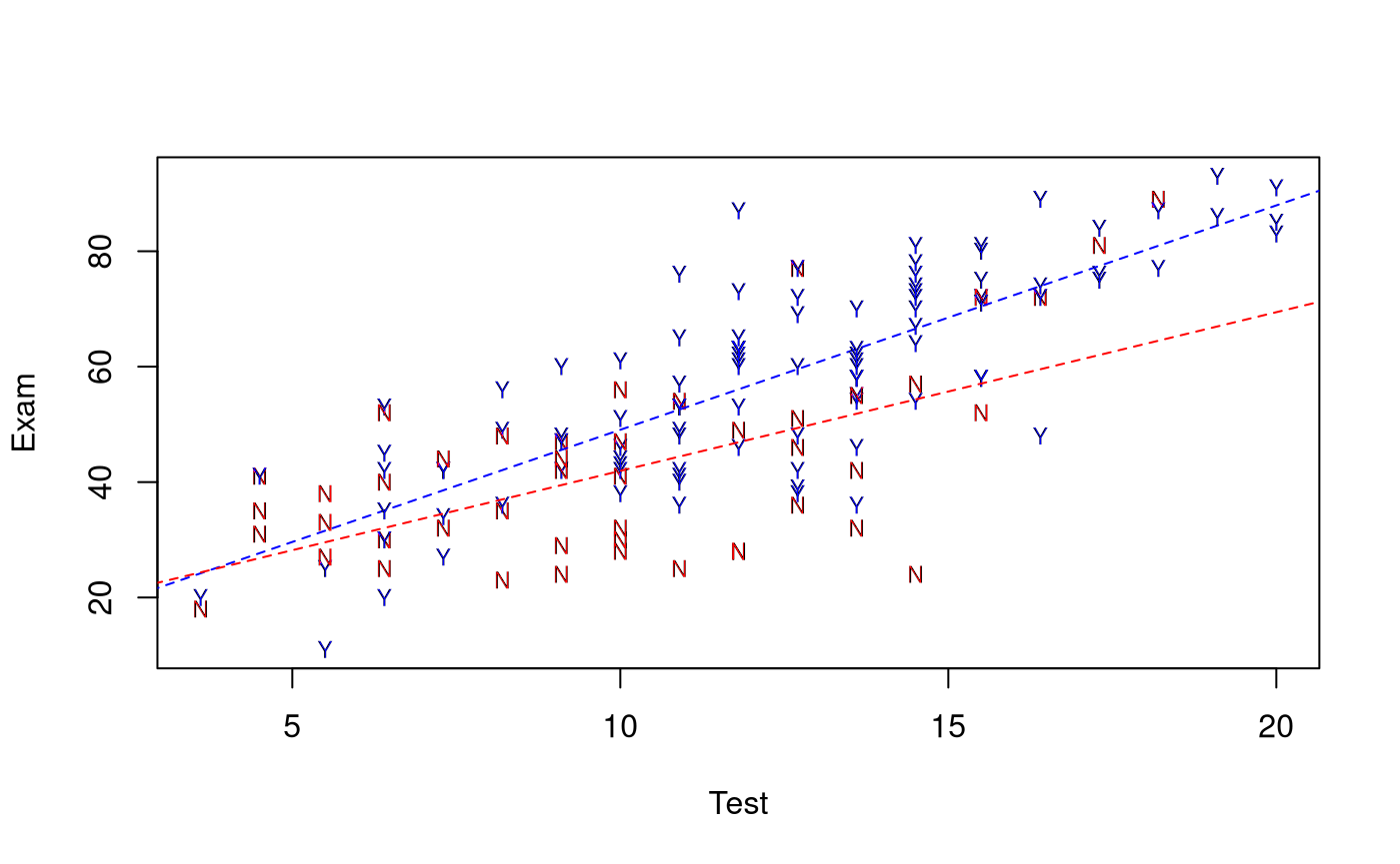

Method and Assumption Checks

As we have two explanatory variables, one numeric and one factor, we have fitted a linear model that used different intercept and slopes for each attendance group (i.e., interaction model). We could not drop the interaction term (P-value = 0.043).

All model assumptions were satisfied.

Our final model is $Exam_i=\beta_0 +\beta_1\times Test_i+ \beta_2\times Attend_i + \beta_3\times Attend_i\times Test_i+ \epsilon_i,$ where $Attend_i=1$ if student $i$ is a regular attender, otherwise 0, and $\epsilon_i \sim iid ~ N(0,\sigma^2)$ .

Our model explained a modest 63% of the variability in students’ exam marks.

Executive Summary

We wanted to quantify students’ exam marks relationship with attendance and test marks.

There was a clear linear relationship between test and exam scores, but this relationship differed between students who attended and who did not attend lectures.

We estimate that each additional test mark (out of 20) obtained by a non-attending student would increase their expected exam mark by between 1.8 to 3.7.

For regular attenders, the increase is an additional 0.04 to 2.24 expected exam marks per test mark.