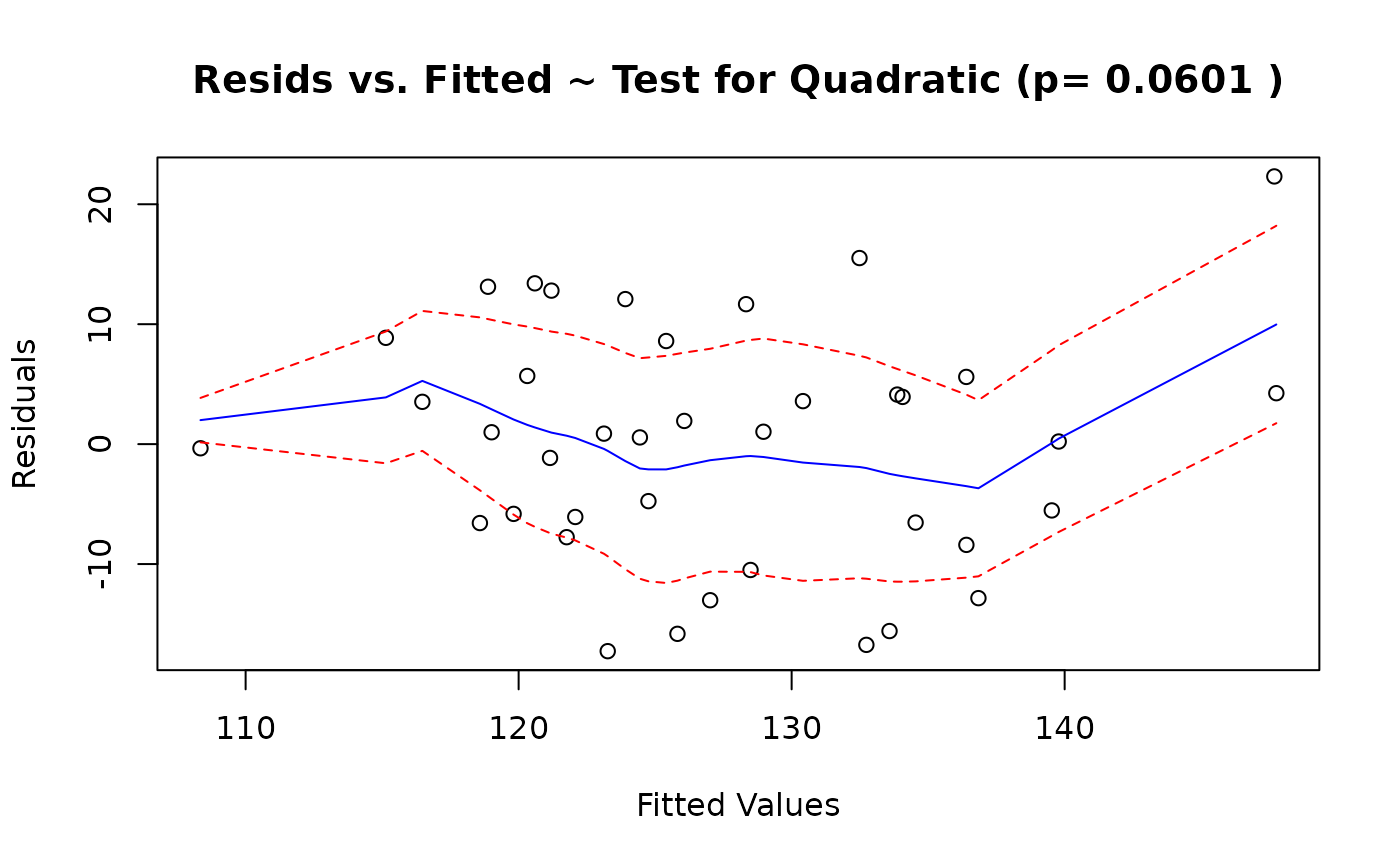
Fitted values versus residuals plot

Plots a scatter plot for the variables of the residuals and fitted values from the linear model, lmfit. A lowess smooth line for the underlying trend, as well as one standard deviation error bounds for the scatter about this trend, are added to this scatter plot. A test for a quadratic relationship between the residuals and the fitted values is also computed.

Usage

residPlot(lmfit, f = 0.5)

Arguments

lmfit: an lm object, i.e. the output from lm.
f: the smoother span. This gives the proportion of points in the plot which influence the smooth at each value. Larger values give more smoothness.

Value

Returns the plot.

Note

This is a legacy diagnostic plotting helper retained for compatibility with older teaching material. New code should usually prefer the current diagnostic workflow used by modelcheck().

Deprecated in s20x 3.4.0. Use modelcheck() instead.

Examples


# Peruvian Indians data
data(peru.df)
fit = lm(BP ~ age + years + weight + height, data = peru.df)
residPlot(fit)
#> Warning: residPlot() is deprecated; use modelcheck() or plot(fit, which = 1) instead.