Case Study 12.1: Exam vs Test & Attendance • s20x

Problem

We wish to determine if regular attendance in class and passing the test is associated with exam mark. We have seen individually that passing the test and regular attendance in class increases the chances for a good exam mark — on average.

The variables of interest are:

Exam: Exam mark out of 100.
Attend: A two-level factor with the levels Yes and No.
Pass.test: A two-level factor with the levels Yes and No.

Question of Interest

We are interested in the relationship between final exam mark and passing the test, and whether this relationship differs for students who did and did not attend lectures regularly.

Read in and Inspect the Data

Stats20x.df = read.table("STATS20x.txt", header = TRUE)

head(Stats20x.df)

##   Grade Pass Exam Degree Gender Attend Assign Test  B  C MC Colour Stage1
## 1     C  Yes   42    BSc   Male    Yes   17.2  9.1  5 13 12   Blue      C
## 2     B  Yes   58   BCom Female    Yes   17.2 13.6 12 12 17 Yellow      A
## 3     A  Yes   81  Other Female    Yes   17.2 14.5 14 17 25   Blue      A
## 4     A  Yes   86  Other Female    Yes   19.6 19.1 15 17 27 Yellow      A
## 5     D   No   35  Other   Male     No    8.0  8.2  4  1 15   Blue      C
## 6     A  Yes   72   BCom Female    Yes   18.4 12.7 15 17 20   Blue      A
##   Years.Since Repeat
## 1         2.5    Yes
## 2         2.0     No
## 3         3.0     No
## 4         0.0     No
## 5         3.0     No
## 6         1.5     No

# So, we have to create the variable `Pass.test' using the `Test` variable
Stats20x.df$Pass.test = factor(ifelse(Stats20x.df$Test >= 10, "pass", "nopass"))
# Check if our new variable `Pass.test` was generated correctly
min(Stats20x.df$Test[Stats20x.df$Pass.test == "pass"])

## [1] 10

max(Stats20x.df$Test[Stats20x.df$Pass.test == "nopass"])

## [1] 9.1

interactionPlots(Exam ~ Pass.test + Attend, data = Stats20x.df)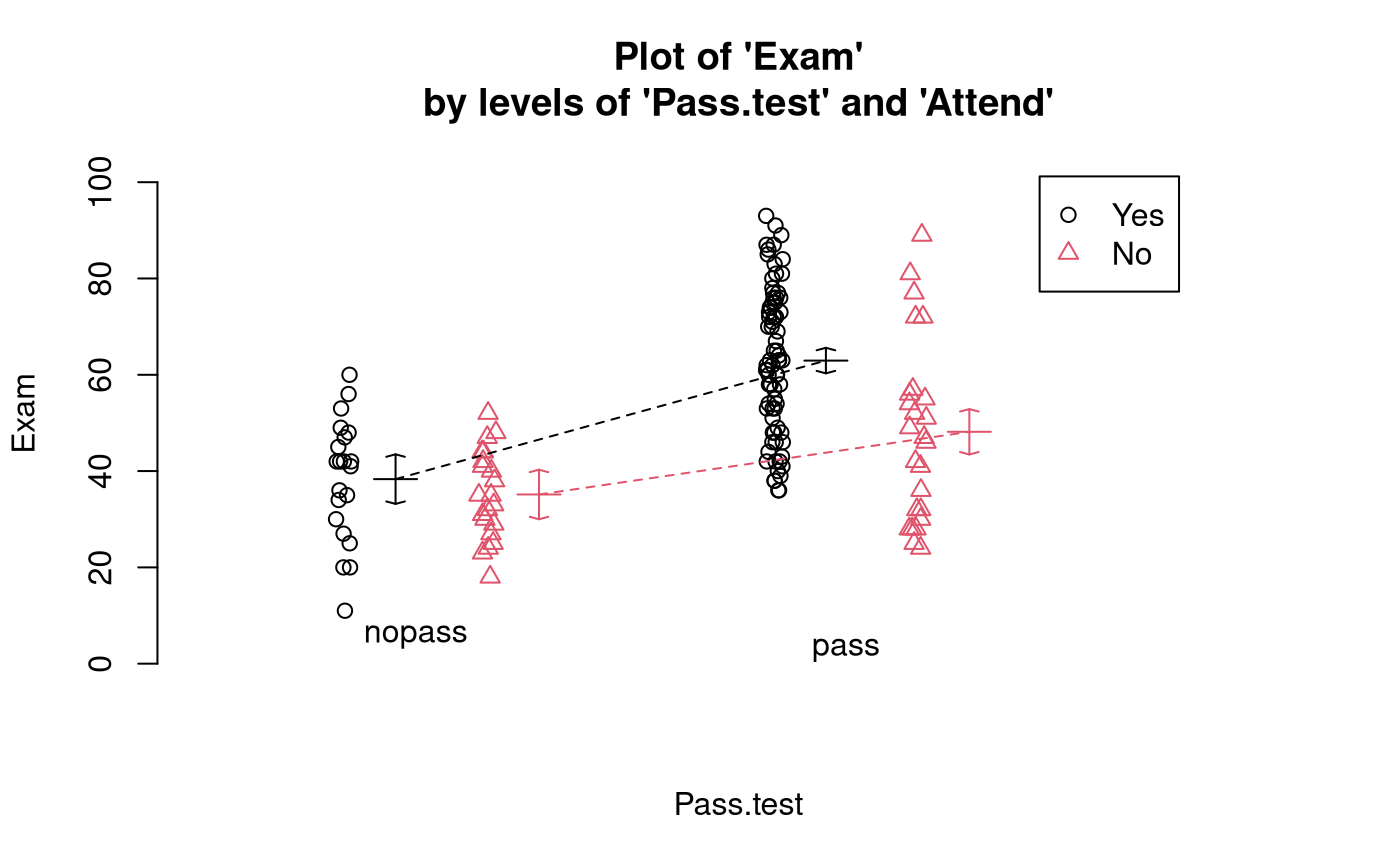

# Also look at the interaction plot the other way around:
interactionPlots(Exam ~ Attend + Pass.test, data = Stats20x.df)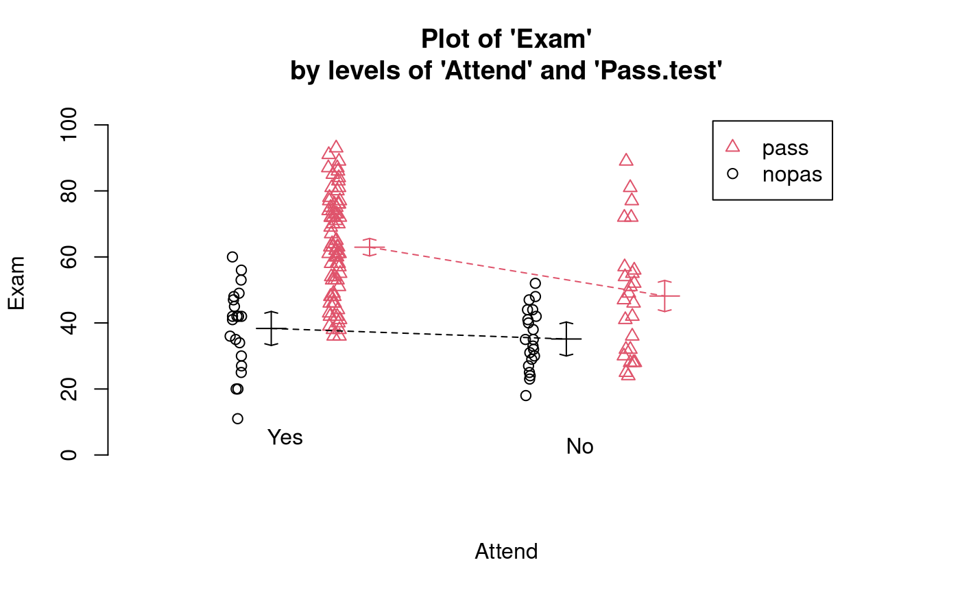

Exam marks for students who passed the test are centred higher than for students who did not. However, this difference appears to be greater for students who attended lectures than for non-attenders, which can be seen from the non-parallel coloured lines on the interaction plots. In other words, the impact of passing the test appears to differ according to attendance group, suggesting there may be an interaction between the two predictor variables.

Model Building and Check Assumptions

Exam.fit = lm(Exam ~ Attend * Pass.test, data = Stats20x.df)
# The model formula could of also been `Exam ~ Attend + Pass.test + Attend:Past.test'
plot(Exam.fit, 1)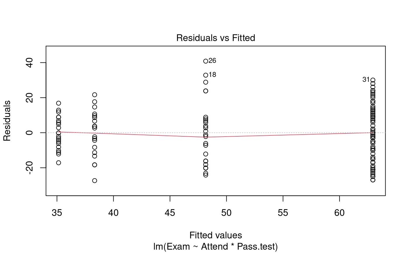

modelcheck(Exam.fit, 2:3)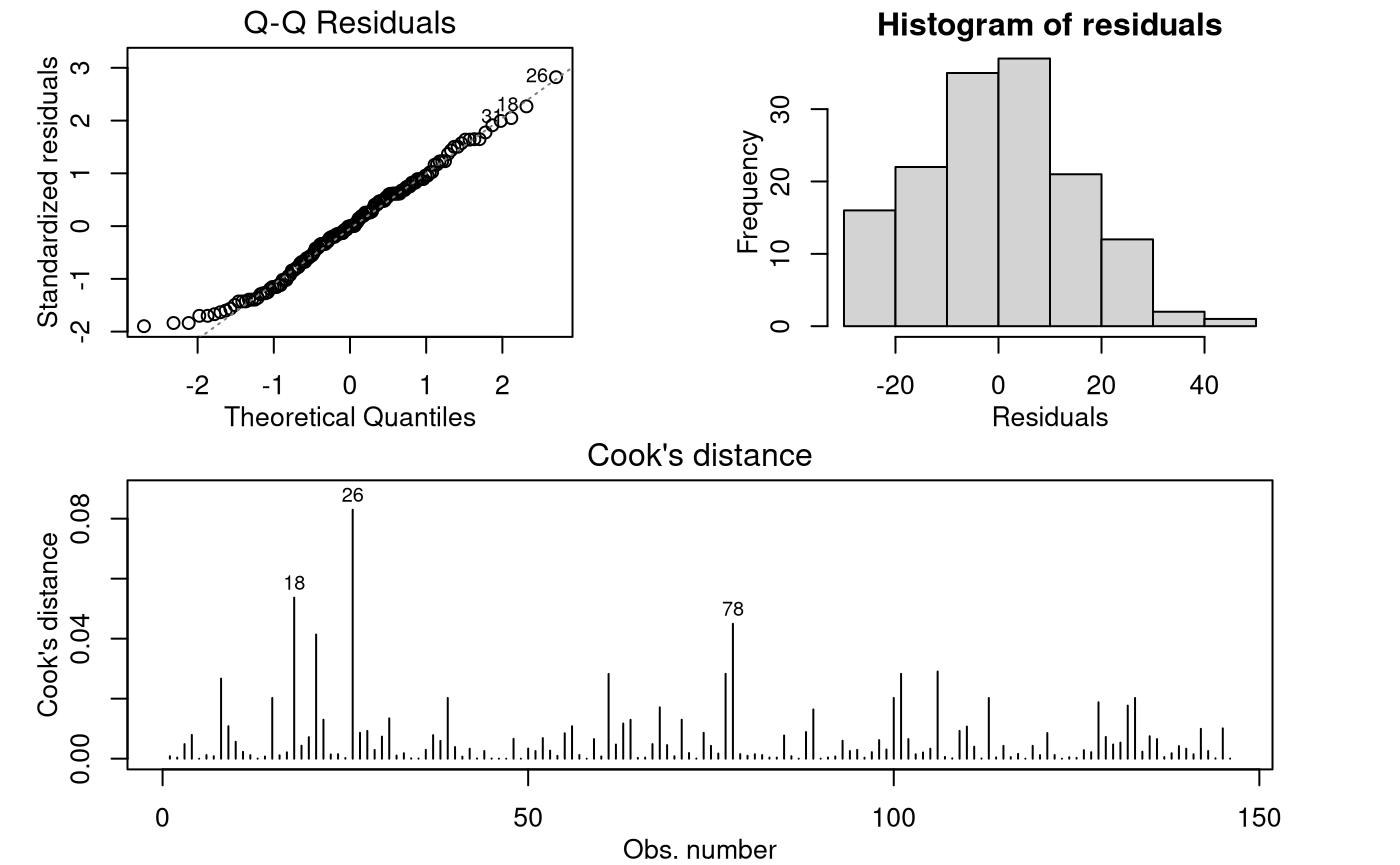

anova(Exam.fit)

## Analysis of Variance Table
## 
## Response: Exam
##                   Df  Sum Sq Mean Sq F value    Pr(>F)    
## Attend             1  7630.8  7630.8  34.990 2.364e-08 ***
## Pass.test          1 11076.9 11076.9  50.791 4.763e-11 ***
## Attend:Pass.test   1   909.7   909.7   4.171   0.04297 *  
## Residuals        142 30968.4   218.1                      
## ---
## Signif. codes:  0 '***' 0.001 '**' 0.01 '*' 0.05 '.' 0.1 ' ' 1

summary(Exam.fit)

## 
## Call:
## lm(formula = Exam ~ Attend * Pass.test, data = Stats20x.df)
## 
## Residuals:
##     Min      1Q  Median      3Q     Max 
## -27.333 -10.893  -0.046   9.513  40.840 
## 
## Coefficients:
##                         Estimate Std. Error t value Pr(>|t|)    
## (Intercept)               35.143      3.223  10.905  < 2e-16 ***
## AttendYes                  3.190      4.557   0.700  0.48504    
## Pass.testpass             13.017      4.371   2.978  0.00341 ** 
## AttendYes:Pass.testpass   11.599      5.679   2.042  0.04297 *  
## ---
## Signif. codes:  0 '***' 0.001 '**' 0.01 '*' 0.05 '.' 0.1 ' ' 1
## 
## Residual standard error: 14.77 on 142 degrees of freedom
## Multiple R-squared:  0.3878, Adjusted R-squared:  0.3749 
## F-statistic: 29.98 on 3 and 142 DF,  p-value: 4.452e-15

Paiwise comparisons

library(emmeans)

## Welcome to emmeans.
## Caution: You lose important information if you filter this package's results.
## See '? untidy'

Exam.pairs = pairs(emmeans(Exam.fit, ~ Attend * Pass.test), infer = TRUE)
Exam.pairs

##  contrast               estimate   SE  df lower.CL upper.CL t.ratio p.value
##  No nopass - Yes nopass    -3.19 4.56 142    -15.0     8.66  -0.700  0.8969
##  No nopass - No pass      -13.02 4.37 142    -24.4    -1.65  -2.978  0.0178
##  No nopass - Yes pass     -27.81 3.63 142    -37.2   -18.38  -7.669 <0.0001
##  Yes nopass - No pass      -9.83 4.37 142    -21.2     1.54  -2.248  0.1155
##  Yes nopass - Yes pass    -24.62 3.63 142    -34.0   -15.19  -6.789 <0.0001
##  No pass - Yes pass       -14.79 3.39 142    -23.6    -5.98  -4.364  0.0001
## 
## Confidence level used: 0.95 
## Conf-level adjustment: tukey method for comparing a family of 4 estimates 
## P value adjustment: tukey method for comparing a family of 4 estimates

# Get a simpler display using displayPairs:
displayPairs(Exam.pairs, c("Yes", "No"), c("pass", "nopass"))

## Note: displayPairs is a s20x function that displays only the within-level
## comparisons from allpairs. To see all comparisons, inspect the allpairs
## output directly.
## 
## $Yes
##               contrast       est       lwr       upr         pval
##  Yes nopass - Yes pass -24.61603 -34.04182 -15.19025 1.701486e-09
## 
## $No
##             contrast       est       lwr       upr       pval
##  No nopass - No pass -13.01714 -24.38137 -1.652912 0.01776097
## 
## $pass
##            contrast       est       lwr       upr         pval
##  No pass - Yes pass -14.78937 -23.59933 -5.979408 0.0001423139
## 
## $nopass
##                contrast       est       lwr      upr     pval
##  No nopass - Yes nopass -3.190476 -15.03851 8.657554 0.896901

Methods and Assumption Checks

We have two explanatory factors, Pass.test and Attend, and one numeric response Exam, so we fitted a two-way ANOVA model with interaction term. The interaction was significant (P-value = 0.04) so it was retained in the model.

The model assumptions seem satisfied.

Our final model is $\text{Exam}_i = \beta_0 + \beta_1 \times Test.pass_i + \beta_2 \times Attend.Yes_i + \beta_3 \times Test.pass_i \times Attend.Yes_i + \epsilon_i,$ where $Test.pass_i$ and $Attend.Yes_i$ are dummy variables that take the value 1 if student $i$ passed the test and if student $i$ regularly attended lectures respectively, otherwise they are 0; and $\epsilon_i \sim iid ~ N(0,\sigma^2)$ .

Alternatively, our final model could be written as $\text{Exam}_{ijk} = \mu + \alpha_i +\beta_j + \gamma_{ij} + \epsilon_{ijk},$ where $\text{Exam}_{ijk}$ is the mark of student $k$ in test-pass group $i$ and attendance group $j$ ; and where $\mu$ is the overall mean exam mark, $\alpha_i$ is the effect of whether the student passed the test, $\beta_j$ is the effect of whether the student regularly attended lectures, $\gamma_{ij}$ is the interaction effect for the combination of a student passing the test and attendance, and $\epsilon_{ijk} \sim iid~N(0,\sigma^2)$ . Here, $i \in \{\text{pass}, \text{ nopass}\}$ and $j \in \{\text{Yes}, \text{ No}\}$ .

Our model explained 39% of variability in students’ exam marks.

Executive Summary

We are interested in the relationship between final exam mark and passing the test, and whether this relationship differs for those students that attended lectures regularly and those that didn’t.

We have evidence that the relationship between exam mark and test-pass status does depend upon attendance practice.

We estimate that:

Among students who attended regularly, the average exam mark for those who passed the test was between 15 and 34 marks higher than for those who didn’t pass the test.
Among students who did not attend regularly, the average exam mark for those who passed the test was between 2 and 24 marks higher than for those who didn’t pass the test.
Among students who passed the test, the average exam mark for those who attended regularly was between 6 and 24 marks higher than for those who didn’t attend regularly.